



An alert fires at 3 a.m.: “response time degradation”. The on-call engineer needs to know straight away whether one service is affected or a whole group of hosts, and whether today’s curve is really unusual compared with last week. The Dynatrace Managed Data Explorer answers all three questions in a few clicks, provided you know what to select.
This practical guide shows how to use the Data Explorer step by step: Build mode, then advanced mode (the metric selector), filters, split by, aggregations, resolution, visualisations, pinning to a dashboard, creating a metric event from a query, sharing and exporting. Each step comes with a concrete operations scenario.
The content targets Dynatrace Managed (builtin: metrics, Metrics API v2 syntax). Dynatrace SaaS also offers the classic Data Explorer, but recent environments rely on Grail and DQL: the queries below do not carry over as they are.
What the Dynatrace Managed Data Explorer is for
The Data Explorer builds metric queries and displays their results. It reads long-term metric data, not traces or individual requests: it is the tool for trends, comparisons and rankings. To isolate one specific slow request, multidimensional analysis is a better fit, and its values can differ from the Data Explorer for that reason.
Typical use cases:
- Saturation: CPU, memory or disk per host, limited to a host group or a management zone.
- Latency and errors: response time and failure rate per service, worst 10 first.
- Period comparison: today against last week with
timeshift. - Derived metrics: an error rate calculated from two counters with an expression.
- Custom and calculated metrics: ingested metrics (StatsD, Prometheus, Telegraf, Metrics API) or calculated service metrics (
calc:service.), queried like built-in metrics. - Preparing a dashboard or an alert: the validated query becomes a tile or a metric event.
Prerequisites
- A Dynatrace Managed environment with OneAgent on the hosts and services to analyse.
- Consistent management zones and host groups: they are your best filters (see the Dynatrace Managed metrics learning path).
- To reuse a query in a script: an access token, which the Copy request action lets you generate through Get a token.
Step by step: a first query in Build mode
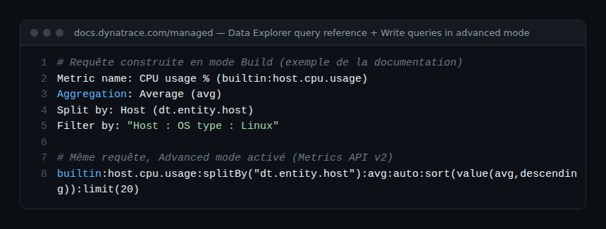
Build mode (Build tab, advanced mode off) assembles the query from menus. Example: CPU of Linux hosts.
- Open Data Explorer. The Start with a template section offers ready-made queries; start from scratch instead.
- In Select metric…, type
cpu usageand pick CPU usage % (builtin:host.cpu.usage) in the Host category. Metrics favourited in the Metrics browser appear at the top of the list; hover over a metric to read its description. - Choose the aggregation: Average.
- Add Split by → Host to get one series per host.
- Add Filter by → Host → OS type → Linux.
- Select Run query. The button shows the time of the last run, or flags unapplied changes.
Then turn on Advanced mode: the same query appears in the exact form passed to the Metrics API v2.
A query holds up to 10 rows (Add metric). Each row has a letter (A, B…): select it or the eye icon to hide the row without deleting it. A row’s More (…) menu offers Duplicate, Delete and Add metric event. Row order matters: the last row is drawn on top and the order sets the column order of a table.
Filters, split by, aggregations and other transformations
A row’s + button adds or removes its transformations. Here is what each one does.
| Transformation | Effect | Values |
|---|---|---|
| Aggregation (space aggregation) | How data points are combined across dimensions | Auto, Average, Count, Maximum, Minimum, Sum, Median, Percentile 10th, 75th, 90th |
| Split by | One series per dimension value; the aggregation applies after the split | Metric dimensions |
| Filter by | Narrows the scope (default: everything); several filters allowed | Dimension → attribute → value |
| Sort by | Series order, descending by default | ASC, DESC |
| Limit | Number of series shown (20 by default) | 1, 10, 20, 100 |
| Rate | Brings a counter to a cadence | None, Per second, Per minute, Per hour |
| Default | Value used when data is missing | Number |
| Timeshift | Shifts the queried timeframe | Positive or negative number + unit (second to week) |
Auto-extended filters use the Smartscape topology: a host metric such as builtin:host.cpu.usage has no host group dimension, yet the Host Group (isInstanceOf) filter still limits it to the hosts of one group. The same principle applies to EC2 instance (runsOn) or to filtering a synthetic step by monitor.
The resolution (time-axis granularity) is set in the Settings panel, to Auto or a value from the list, for graphs, stacked columns and areas, heatmaps and histograms. The finest resolution is one minute.
Concrete scenarios
CPU per host group
Metric builtin:host.cpu.usage, Average aggregation, split by Host, Host Group (isInstanceOf) filter on the group you want, Graph visualisation. For a per-team dashboard, pin the tile without a group filter and add a dynamic filter to the dashboard: auto-extended filters also work at dashboard level. Host metrics are covered in the hosts and infrastructure module.
Response time per service, top 10
builtin:service.response.time:splitBy("dt.entity.service"):percentile(90):sort(value(percentile(90),descending)):limit(10)Top list or Table visualisation. Watch out: the unit of builtin:service.response.time is the microsecond. Add a second row builtin:service.errors.total.rate (percent, auto and avg aggregations) to cross latency with errors. The service metrics module lists the other useful keys.
Compare with last week
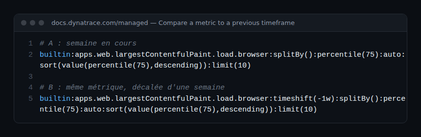
Duplicate the row (More → Duplicate), switch to advanced mode and append :timeshift(-1w) to the copy. Both curves overlap: a spike that already existed the week before is often a scheduled job, not an incident.
A calculated error rate
In advanced mode, an expression combines operands (metrics or numbers) in parentheses with + - * /. For a percentage: ((A)/(B))*(100), where A and B are two full selectors, for example builtin:apps.web.action.countOfErrors and builtin:apps.web.action.count.load.browser filtered on the same page. All metrics in an expression must have the same resolution.
Filter by tag or related entity
builtin:host.cpu.usage:filter(in("dt.entity.host",entitySelector("type(HOST),tag(~"env:prod~")"))):splitBy("dt.entity.host"):avgThe in() filter accepts an entity selector: tag, management zone (mzName()) or relationship (toRelationships, fromRelationships). That is how you limit, for example, a Kubernetes node metric to one cluster.
Choosing the visualisation
- Graph: series over time, as line, column or area per metric (up to 20 series per metric). The only visualisation offering baseline, correlated metrics and focus.
- Stacked column / Stacked area: stacking, only for metrics with the same unit.
- Single value: one aggregated value, with trend, sparkline and threshold background.
- Table: one column per metric, 100 rows by default, thresholds per metric.
- Top list: ranking of a single metric.
- Pie, Heatmap, Honeycomb (one cell per result, coloured by threshold) and Histogram (metrics whose key ends in
.histogram).
On a graph, select a line: Add baseline draws a confidence band, See correlated metrics asks Davis for series with a similar shape (a split by is required), Focus hides the rest. Baseline and focus are not carried over to the pinned tile.
Pin, alert, share
- Pin to dashboard: choose an existing dashboard or Create new dashboard. It is the only way to save a query: leaving the Data Explorer discards it. To edit later, tile menu → Configure tile in Data Explorer, then Save changes to dashboard. See the Managed dashboards guide.
- Add metric event (row More menu): Settings → Anomaly detection → Metric events opens in a new window with the metric fields pre-filled. Complete the threshold or baseline, then save. The metric selector and alerts module details these settings.
- Share link (Result section menu): turn on Use the current timeframe to freeze the period, otherwise the link carries the query without the timeframe. Only authenticated users can open it.
- Export CSV and Copy request: the first exports formatted values, the second copies the API call (JSON or CSV response), ready for a script.
How to check that it works
After Run query, the button shows the time of the last run. Open Copy request: the query shown is the one actually sent, fallback transformation included. On the dashboard, the pinned tile must show the same series as the Data Explorer for the same timeframe.
Common pitfalls and limits
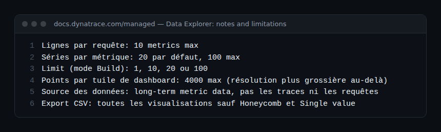
- Missing series: 20 by default, 100 at most. Filter (management zone, entity name) rather than raising the limit.
- Empty table cells: each metric returns its own top. Set the Global limit on the reference metric to align rows.
- Dip at the end of the curve: the last interval is incomplete. Remove one or two buckets from the timeframe, for example
-2h-2minstead of-2h. - Tile coarser than the Data Explorer: a tile returns at most 4,000 data points; beyond that, the resolution becomes coarser.
- No way back to Build mode: after adding a
timeshiftor an expression in advanced mode, you cannot switch back to Build mode. - Availability differs from the Hosts page:
builtin:host.availabilityrelies on time series, the Hosts page on dedicated events.
Best practices
- Start in Build mode, then read the query in advanced mode: it is the best way to learn the metric selector.
- For latency, prefer a percentile (90th) over the average, which hides the slow tail.
- Filter by management zone before raising the limit: fewer series, faster answers.
- Rename rows (Rename) before pinning: the original metric name stays in the query.
- Validate a query over 7 days in the Data Explorer before turning it into a metric event, to limit false alerts and on-call toil.
Frequently asked questions
Does the Data Explorer save my queries?
No. A query that is not pinned is lost when you leave the page. Pin it to a dashboard or keep a share link.
Why do my numbers differ from multidimensional analysis?
The Data Explorer reads long-term metrics, multidimensional analysis reads request and trace data. Aggregations and granularity are not the same.
Can I query my custom metrics?
Yes. Metrics ingested via StatsD, Prometheus, Telegraf or the Metrics API, as well as calc:service. calculated metrics, appear in the selection list and accept the same transformations.
Conclusion
The Dynatrace Managed Data Explorer covers the full cycle of a metric-based investigation: explore in Build mode, refine with the metric selector, compare over time, then turn the query into a tile or a metric event. Used well, it shortens MTTR and makes alerts more accurate. Official reference: Data Explorer, Dynatrace Managed documentation and Write queries in advanced mode.
span.observer is an independent community blog, not affiliated with Dynatrace LLC. Dynatrace is a trademark of its owner. Examples are provided for guidance only: check them against the official documentation for your version.